The intricate atomic, molecular, and cellular order observed in living beings, juxtaposed with their inanimate counterparts, stands as a notable commonality. Yet, it is imperative to acknowledge that physical laws make no distinction between living and non-living entities. In this discourse, highlighting the profound significance of the second law of thermodynamics assumes paramount importance. This foundational law dictates an inexorable increase in total disorder, posing a formidable challenge to maintaining order within an environment governed by its principles. Molecules tend to disperse and degrade, cells inevitably age and expire, necessitating a continuous replenishment to sustain life. Thus, living organisms expend energy and introduce a higher level of disorder in their surroundings compared to the order they intricately construct within themselves.
Consider, for instance, the erythrocytes ferrying oxygen from the lungs to the brain, with a fleeting lifespan of a mere two months. Thankfully, the breakdown of consumed nutrients provides the energy and disorder required for timely replacements. However, unlike other cells, the neurons in the brain lack the capacity to proliferate, thereby necessitating the preservation of vitality throughout one’s lifespan. Yet, vitality alone fails to safeguard cognitive faculties; the intricate cellular order forged by the amalgamation of neurons must also remain undisturbed. Naturally, this endeavor demands continual energy acquisition from the environment, perpetuating disorder within it.
A living organism cannot persist indefinitely far from equilibrium with its environment, even if it expands or modifies its surroundings. Once it succumbs to the pervasive influence of the fundamental premise of thermodynamics, colloquially known as “molecular chaos,” [Note 1] it swiftly converges towards equilibrium with its environment. Any semblance of correlation among atoms and molecules disappears, aligning inexorably with the second law of thermodynamics, and thereby extinguishing its vitality.
As discerned, the quantification of disorder, particularly from a scientific perspective, assumes a significance akin to a matter of existential importance. However, should this argument fail to elicit further inquiry, I humbly suggest reviewing Note 2 before proceeding.
Representation of Molecular and Atomic Disorder
To accurately gauge disorder within a system, it is imperative to delineate the physical state of that system mathematically. One of the most prevalent tools employed for this purpose is the concept of “probability distribution.” The ensuing discussion shall exclusively focus on elucidating this concept, endeavoring to comprehend the probabilistic essence of disorder and exploring avenues for its mitigation, all through the lens of the water – a molecular system simpler than living systems yet undeniably indispensable for life.
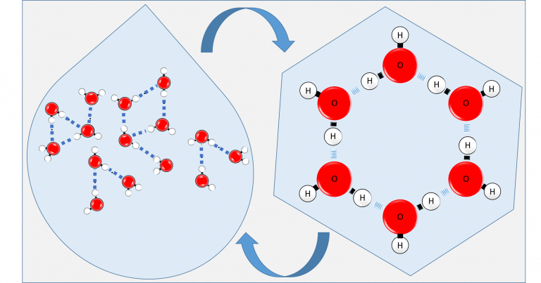
Let us embark upon an exploration of the molecular architecture of water. A water molecule (H2O) manifests through the strong chemical bonding of two hydrogen (H) atoms with one oxygen (O) atom, known as covalent bonds. In Figure 1, which illustrates a molecular cluster consisting of 15 water molecules, hydrogen and oxygen atoms are depicted as white and red spheres, respectively, while the covalent bonds are represented by small black rods. It is worth noting that intermittent blue dashed lines indicate interactions between water molecules in this depiction. These interactions, known as hydrogen bonds, represent weaker chemical bonds compared to covalent bonds.
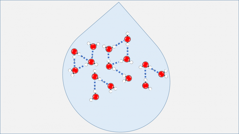
Figure 1: Water Molecules in Liquid State. Red spheres represent oxygen (O), while white spheres represent hydrogen (H) atoms. The dark blue dashed lines connecting oxygen and hydrogen atoms of different H2O molecules represent hydrogen bonds.
A single water molecule has the capacity to form hydrogen bonds with up to 4 different water molecules concurrently. However, the kinetic energy inherent in molecules at temperatures above 0°C often facilitates the rupture of these bonds. Consequently, the fluidity of water at such temperatures, rather than a solid state, is underpinned by the facile breaking and reforming of hydrogen bonds between molecules.
When examining a water molecule in relation to surrounding molecules, there are five distinct scenarios we may observe regarding the number of hydrogen bonds it forms:
– Absence of hydrogen bonds
– Single hydrogen bond
– Double hydrogen bonds
– Triple hydrogen bonds
– Quadruple hydrogen bonds
In this context, the molecular disorder of water at a constant temperature T can be roughly elucidated by the probability distribution of the number of hydrogen bonds a randomly selected water molecule may exhibit, denoted as “p” [Note 3]:
p(T) = (p4, p3, p2, p1, p0)
Whereby a chosen water molecule may possess four hydrogen bonds with probability p4, three hydrogen bonds with probability p3, two hydrogen bonds with probability p2, one hydrogen bond with probability p1, and 0 hydrogen bonds with probability p0. Thus, the probability distribution corresponding to maximal disorder is as follows:
p(Tmax) = (1/5, 1/5, 1/5, 1/5, 1/5)
Consequently, each water molecule, on average, harbors 2 hydrogen bonds: (4+3+2+1+0)/5 = 2. At lower temperatures, such as room temperature, between 20–25°C, this number escalates to 3.4 [Note 4]. For instance, we may derive distributions such as:
p(Troom; 1) = (3/5, 1/5, 1/5, 0, 0)
or
p(Troom; 2) = (2/5, 3/5, 0, 0, 0)
Both distributions denote diminished disorder compared to p(Tmax): overall randomness regarding the number of hydrogen bonds decreases, and predictability increases. When water is cooled to 0°C, indicating the transition from liquid to solid state, molecular disorder gives way to maximum order, where each molecule forms four hydrogen bonds, as partially depicted in Figure 2:
p(Tice) = (1, 0, 0, 0, 0)
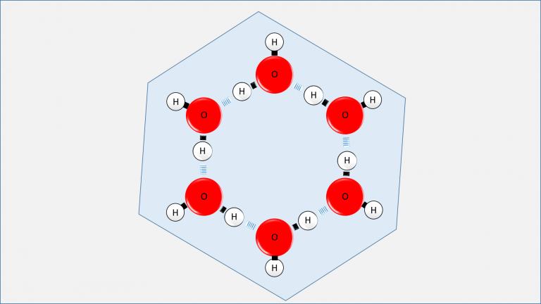
Figure 2: Six water molecules present only on one surface of a unit cell in hexagonal ice. You can imagine the entire molecular structure folded together like a chair or a boat on each surface, forming a three-dimensional crystal. In this three-dimensional structure, each water molecule will form hydrogen bonds with four different water molecules.
At this juncture, all oxygen atoms are immobilized in their current positions. However, the hydrogen atoms, owing to their substantially smaller mass, possess the capability to hop from one molecule to another via hydrogen bonds until extremely low temperatures are reached. Consequently, a randomly selected water molecule within the ice could assume any of the six distinct bonding configurations depicted in Figure 3. Thus, transitioning from the molecular to atomic scale, we encounter yet another layer of disorder.
Similar to the preceding, we can delineate this atomic disorder by outlining the distribution of the probability of a randomly selected molecule occupying each depicted state in Figure 3, denoted as “q”:
q(T) = (q1, q2, q3, q4, q5, q6)
At 0°C, where the likelihood of being in each state is equal, the atomic disorder peaks:
q(0°C) = (1/6, 1/6, 1/6, 1/6, 1/6, 1/6)
As the temperature decreases, so too does atomic disorder. In fact, just below -200°C, all molecules reside in only one possible configuration, such as the first one [Note 5]:
q(-200°C) = (1, 0, 0, 0, 0, 0)
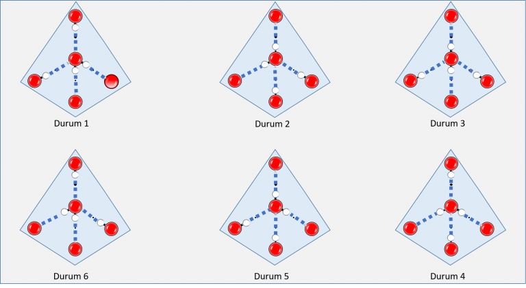
Figure 3: Possible bonding configurations of a water molecule forming four hydrogen bonds (illustrated with blue dashed lines). For simplicity, the depiction excludes hydrogen atoms (depicted as white spheres) of other water molecules surrounding this central molecule.
After attaining molecular order, the excessively cooled water molecules proceed to achieve atomic order as well. Consider for a moment the staggering electricity bill if your refrigerator were to consume such a vast amount of energy. As expected, the cost of creating such order in water is significant. However, within living cells, even at body temperature, these atomic and/or molecular orders can be achieved on small clusters of water [Note 6]. Subsequently, they have the ability to disrupt the order among water molecules and establish another atomic and/or molecular order within themselves amidst the resulting disorder.
Further Mathematical Considerations
In forthcoming discussions, I aim to introduce you to various measures of disorder such as entropy and majorization. Through this exploration, the concept of disorder elucidated by probability distributions, as mentioned earlier, will become more tangible. We shall observe that the disorder quantities described by probability distributions such as p(Tmax), p(Troom; 1), and p(Troom; 2) translate to entropy values of 2.32, 1.37, and 0.97, respectively. Utilizing the majorization relationships between these distributions, we shall also examine the feasibility of transitions between them. But for now, let us pause here and take a moment to reflect. The next post will focus on the contextuality of the probabilistic description of a physical system’s state. Following that, we’ll focus on quantum probabilities in the subsequent post.
Stay engaged with the realm of science.
Onur Pusuluk
Notes:
[1] To better understand what is meant by “molecular chaos” in the text, you can refer to the link below, especially the second paragraph provided there:
https://en.wikipedia.org/wiki/Molecular_chaos
[2] The crucial role that disorder plays in determining the inevitable fate we face, may not have fully convinced everyone of the necessity to quantify it mathematically. Nevertheless, I can assure you that the second law of thermodynamics isn’t confined to biology alone; its application extends across diverse fields, from physics and chemistry to mechanical and communication engineering, and even economics. Many significant calculations in our lives necessitate measuring disorder. Some examples that come to mind include:
– assessing the maximum energy efficiency of everyday appliances like your kitchen’s water heater, refrigerator, or the motor vehicle you rely on for daily commuting,
– determining the maximum achievable compression for files stored on your computer, videos uploaded to the internet, or messages sent from your cell phone,
– analyzing income inequality within a nation and comparing the welfare levels of different countries based on this metric.
Perhaps in another post, we could explore these topics in greater detail.
[3] Of course, this temperature should be lower than a certain upper limit below 100 °C. Because at temperatures where the (thermal) kinetic energies of molecules are much larger than the energies of hydrogen bonds between them, we cannot define disorder based on the number of hydrogen bonds. Remember that when water is heated to 100 °C, all hydrogen bonds will break, so in a sense, the transition from the liquid phase to the gas phase will occur.
[4] This number can be found in almost all biochemistry and biophysics textbooks when discussing the structure of water. However, I currently do not know what the original source is.
[5] Molecules can transition from one state to another, such as from the first state to the second state in Figure 3, due to quantum mechanical phenomena such as quantum tunnelling or quantum superposition even below –200 °C. However, this does not change the fact that when we make a measurement, they will all be in the same state. Therefore, the order/disorder of molecules remains unchanged.
[6] “Confined water” within living cells is different from ordinary liquid water in many ways and can sometimes exhibit certain properties specific to water ice, such as atomic and molecular arrangements.